(You may see the rest of the lecture notes here).

Office: WWH 921

Office hours: after each class, 11 am - noon, or by appointment

There will be weekly problem sets posted that are worth 0 points but are meant as study guidance.

There will be a midterm exam (oral exam, done between October 15th and Oct 22), and a final exam (also oral). They are worth 40% and 60% of the course grade, respectively. Each exam should be about 20 mins.

I am expecting to not have to take attendance. I will be posting a problem set to give you practice and guide office hour discussions.

“Optimal transport” is a field of mathematics & an array of tools used throughout engineering and science.

It’s concerned with maps that preserve volume and/or ways of “matching” two distributions together, and this “transport”/“matching” is optimal in some sense.

Optimal transport

The discrete problem

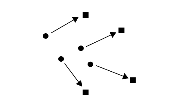
Consider two sets of points on the plane, $X$ (squares) and $Y$ (circles).

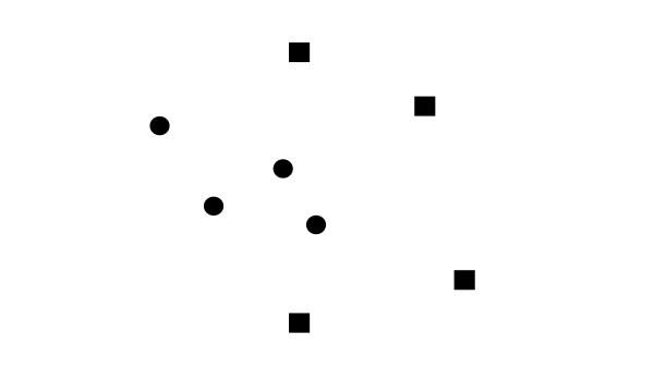
The transportation cost from $x \in X$ to $y\in Y$ is denoted $c(x,y)$.

\[c:X\times Y\mapsto \mathbb{R}\]

Problem. Find a bijective function (a “map”) $T: X\mapsto Y$ minimizing the “total transportation cost” $\mathcal{C}(T)$, given by

\[\mathcal{C}(T) = \sum \limits_{x\in X} c(x,T(x))\]

As $X$ and $Y$ are finite, there are finitely many choices, so at least one of them achieves the smallest value

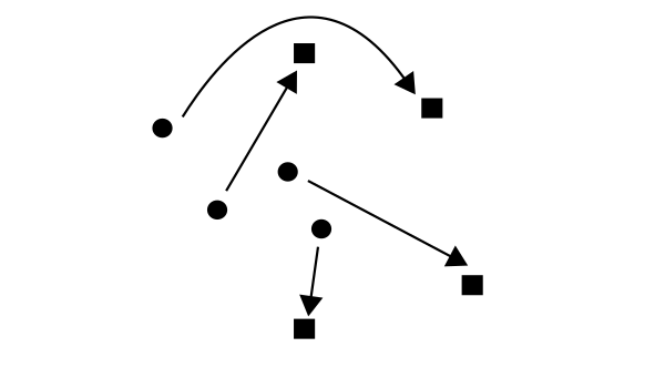
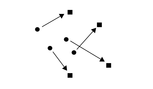
Let $T$ be an optimal transport map. Then, if $n>0$, $x_1,\ldots,x_n$ are points in $X$, and $\sigma$ is a permutation of ${1,\ldots,n}$,

\[\sum \limits_{k=1}^N c(x_k,y_k) \leq \sum \limits_{k=1}^N c(x_k,T(x_{\sigma(k)}))\]

SPOILER ALERT: This is a very strong property! A theorem of Rockafellar says (morally) that if \(c(x,y)=\|x-y\|^2\), then there is a function $u:\mathbb{R}^2\to\mathbb{R}$ such that for every $x\in X$ we have

\[T(x) = \nabla u(x)\]

and what’s more: $u$ is a convex function (more on this later).

The continuum problem

In optimal transport in $\mathbb{R}^n$, we are typically concerned with mass densities $f(x)$ and $g(y)$, and transformations

\[T:\mathbb{R}^n\to\mathbb{R}^n\]

which transport the first density to the second, meaning that we ask that

\[\int_Ef(x)\;dx = \int_{T(E)}g(y)\;dy\;\;\forall\;E\subset \mathbb{R}^n\]

(or, alternatively, we may ask that

\[\int_{T^{-1}(E)}f(x)\;dx = \int_{E}g(y)\;dy\;\;\forall\;E\subset \mathbb{R}^n\]

and these conditions are not necessarily the same).

For general measures $\mu$ and $\nu$, the second of these two conditions can be stated as

\[\int_{\mathbb{R}^n}\eta(T(x))\;d\mu(x) = \int_{\mathbb{R}^n}\eta(y)\;d\nu(y),\;\;\forall\;\eta\in C_c^0(\mathbb{R}^n)\]

We may ask to find, for example, for the transport map $T$ from $\mu$ to $\nu$ with the least total quadratic distance $\mathcal{C}(T)$, where

\[\mathcal{C}_2(T) = \int_{\mathbb{R}^n}|x-T(x)|^2\;d\mu(x)\]

At least when $\mu = f\;dx$ and $\nu = g\;dy$ this problem has a minimizer $T(x)$ which is uniquely defined a.e. in the set $\{f>0\}$.

In this manner one defines what is often called the Wasserstein distance, and which we will call here the (quadratic) transport distance,

\[d_2(\mu,\nu) := \left (\inf_T \mathcal{C}_2(T) \right )^{1/2}\]

This turns the space $\mathcal{P}_2(\mathbb{R}^n)$ into a metric space, and more.

Everything is optimal transport

Geometric data processing / information geometry

(A picture of three translates of the same compactly distributed distribution. Which of the two densities in blue is “closest” to the one in red?)

Several metrics to quantify their similarity: $KL$ divergence, $L^p$ distances between the densities, total variation distance, quadratic transport distance.

Of these distances, only the quadratic transport distance distinguishes between the two blue distributions.

The transport distance is the only one that captures the geometry of the densities if we treat them as clouds of random points.

Prescription of Gauss curvature

If $u:D\subset\mathbb{R}^2 \to \mathbb{R}$ solves the PDE,

\[\frac{\det(D^2u(x))}{1+|\nabla u|^2} = K(x)\]

then the graph of $u$ will have Gauss curvature $K(x)$ at the point $(x,u(x))$. This can be thought of as an optimal transport problem from $D\subset \mathbb{R}^2$ to a subset $\overline{D}\subset \mathbb{S}^2$.

Optimal couplings of random variables

Given two mean zero random variables $X,Y$, find a joint law $\pi$ for $(X,Y)$ which maximizes their covariance,

\[\mathbb{E}_\pi[X\cdot Y]\]

Variational inference

Suppose we have a parametric family of probability densities $\mu_\theta$, $\theta \in \mathbb{R}^p$, and we are given a “target” measure $\mu$.

Then, often times we are interested in understanding the member of the family $\mu_\theta$ closest to $\mu$ in the transport distance,

\[\text{argmin}_\theta d_2(\mu_\theta,\mu)\]

Interpolation and barycenters

The usual (vector space of signed measures) interpolaton of measures does not capture the underlying geometric structure.

\[\text{argmin}_\mu \left \{ \frac{1}{2}d(\mu,\mu_1)+\frac{1}{2}d(\mu,\mu_2) \right \}\]

The power of OT, via three examples

Example I: The isoperimetric inequality

Theorem.

Given $E \subset \mathbb{R}^n$, if $|E|$ denotes its volume, and $|\partial E|$ denotes its perimeter, then $$ \frac{|\partial B|^{\frac{n}{n-1}}}{|B|} \leq \frac{|\partial E|^{\frac{n}{n-1}}}{|E|} $$

Take any ball $B$ of volume equal to $E$. As it turns out, optimal transport says there exists a one-to-one volume-preserving transformation $T:E\to B$. What is more, this transformation has a very special structure: there exists a convex function $u:\mathbb{R}^n\to \mathbb{R}$ such that

\[T(x) = \nabla u(x) \text{ for every } x\in E\] \[|B| = \int_{B}1\;dx = \int_{E}1\cdot\det(DT(x))\;dx\]

Now, $DT(x) = D^2u(x)$, and $u$ being convex, $D^2u(x)$ is a positive semi-definite matrix for every $x\in E$. Then, the arithmetic-geometric mean inequality says that

\[\det(DT(x))^{\frac{1}{n}} = (\det(D^2u(x)))^{\frac{1}{n}} \leq \frac{1}{n}\Delta u(x).\]

Now,

\[|B| = \int_{E}(\det(D^2u(x)))^{\frac{1}{n}}\;dx \leq \frac{1}{n}\int_{E}\Delta u(x)\;dx\]

The right hand side is simply begging to be rewritten using the divergence theorem, and so we have

\[|B| \leq \frac{1}{n}\int_{\partial E}\nabla u(x)\cdot n(x) \;d\sigma(x)\]

The map $\nabla u$ maps $E$ onto $B$, a ball of radius $r$, and so $

\nabla u(x)

\leq r$ for every $x$, and so

\[|E| = |B| \leq \frac{1}{n}\int_{\partial E}r\;d\sigma(x) = \frac{r}{n}|\partial E|\]

On the other hand,

\[|E| = |B| = \omega_n r^n \Rightarrow r = \left ( \frac{|E|}{\omega_n} \right )^{\frac{1}{n}}\]

Therefore,

\[|E| \leq \frac{|E|^{\frac{1}{n}}}{n\omega_n^{\frac{1}{n}}}|\partial E|\]

Rearranging,

\[n\omega^{\frac{1}{n}}|E|^{\frac{n-1}{n}} \leq |\partial E|, \text{ or } n\omega^{\frac{1}{n}} \leq \frac{|\partial E|}{|E|}^{\frac{n-1}{n}}\]

Example 2: Parabolic PDE and minimizing movements.

An important PDE is the porous medium equation, which depends on a parameter $m\geq 1$, and is given by

\[\partial_t \rho = \Delta \rho^m\]

Suppose you are given an initial mass density $\rho_0$. Fix $h>0$, and then consider the minimization problem

\[\min_\rho \left \{ h\int_{\mathbb{R}^n} \rho^p\;dx + \frac{1}{2}d_2(\rho,\rho_0)^2\right \}\]

and this way, we can generate iteratively a sequence $\rho_k$, $k=0,1,2,\ldots$.

Define $\rho^{(h)}(x,t)$ to be a step function in time, which equals $\rho_k$ if $t\in [hk,h(k+1))$.

Theorem. (Felix Otto, ~2000)

The sequence $\rho^{(h)} $ converges as $h\to 0$ to $\rho(x,t)$, the unique weak solution to the Cauchy problem $$\partial_t \rho = \Delta \rho^m,\;\rho(x,0+) = \rho_0(x)$$

The limiting case as $m \to 1^+$ takes us to the heat equation. A follow up paper by Jordan, Kinderlehrer, and Otto applied the above framework to the Fokker-Planck, or Langevin equation.

\[\partial_t \rho = \text{div}(\nabla \rho + \rho \nabla V)\]

The JKO scheme says that to solve this equation, one may succesfully solve the variational problem

\[\min_\rho \left \{ h\int_{\mathbb{R}^n}f\log(f/g)\;dx + \frac{1}{2}d_2(\rho,\rho_{k})^2\right \}\]

where $g = Z^{-1}e^{-V}$. If $V$ is $\alpha$-convex, one can show that

\[\text{KL}(\rho(t),g)\leq e^{-\alpha t}\text{KL}(\rho(0),g)\]

and so we converge (in the KL metric) to $g$ with an exponential rate.

Example 3: OT and curvature in a Riemannian manifold

*Explain, roughly, what Ricci curvature is.

Displacement interpolation, given two measures $\mu_0$ and $\mu_1$, we can find a curve $\mu_t$, $t\in [0,1]$ such that

\[d_2(\mu_t,\mu_0) = d_2(\mu_1,\mu_0)t\]

A combination of theorems of Lott-Villani and Sturm says that a manifold has non-negative Ricci curvature if and only if the Boltzmann entropy functional is displacement convex in the space $P_2(M)$ equipped with the transport metric.

A word from our sponsor: $\det(D^2u) = f$

If $\nabla u(x)$ maps a density $f$ to a density $g$, then the change of variables formula says that

\[\det(D^2u(x)) = \frac{f(x)}{g(\nabla u(x))}\]

Indeed, if for every $E$ we have,

\[\int_Ef(x)\;dx = \int_{\nabla u(E)}g(y)\;dy\]

then, the change of variables $y=\nabla u(x)$ says that

\[\int_Ef(x)\;dx = \int_E g(\nabla u(x))\det(D^2u(x))\;dx\]

This connects the regularity of the optimal transport map $T(x)=\nabla u(x)$ to the regularity of $u$, which solves a scalar, nonlinear PDE.